PyTorch的简洁设计使得它入门很简单，在深入介绍PyTorch之前，本节将先介绍一些PyTorch的基础知识，使得读者能够对PyTorch有一个大致的了解，并能够用PyTorch搭建一个简单的神经网络。

Tensor

Tensor是PyTorch中重要的数据结构，可认为是一个高维数组。它可以是一个数（标量）、一维数组（向量）、二维数组（矩阵）以及更高维的数组。Tensor和Numpy的ndarrays类似，但Tensor可以使用GPU进行加速。Tensor的使用和Numpy及Matlab的接口十分相似。（与Tensorflow中的Tensorflow基本相同）

构建 5x3 矩阵，只是分配了空间，未初始化

# 构建 5x3 矩阵，只是分配了空间，未初始化
x = t.Tensor(5, 3)  
[output]:
1.00000e-07 *
  0.0000  0.0000  5.3571
  0.0000  0.0000  0.0000
  0.0000  0.0000  0.0000
  0.0000  5.4822  0.0000
  5.4823  0.0000  5.4823
[torch.FloatTensor of size 5x3]

使用[0,1]均匀分布随机初始化二维数组

# 使用[0,1]均匀分布随机初始化二维数组
x = t.rand(5, 3)  
[output]:
0.3673  0.2522  0.3553
 0.0070  0.7138  0.0463
 0.6198  0.6019  0.3752
 0.4755  0.3675  0.3032
 0.5824  0.5104  0.5759
[torch.FloatTensor of size 5x3]

查看x的形状(torch.Size 是tuple对象的子类，因此它支持tuple的所有操作，如x.size()[0])

# 查看x的形状
x.size()[1], x.size(1) # 查看列的个数, 两种写法等价

Tensor的加法

x = t.rand(5, 3)  
y = t.rand(5, 3)
# 加法的第一种写法
x + y
# 加法的第二种写法
t.add(x, y)
# 加法的第三种写法：指定加法结果的输出目标为result
result = t.Tensor(5, 3) # 预先分配空间
t.add(x, y, out=result) # 输入到result

 # 普通加法，不改变y的内容
y.add(x)
print(y)

# inplace 加法，y变了
y.add_(x) 
print(y)

注意：函数名后面带下划线_ 的函数会修改Tensor本身。例如，x.add_(y)和x.t_()会改变 x，但x.add(y)和x.t()返回一个新的Tensor，而x不变。

Tensor的选取操作与Numpy类似。Tensor和Numpy的数组之间的互操作非常容易且快速。对于Tensor不支持的操作，可以先转为Numpy数组处理，之后再转回Tensor

# Tensor的选取操作与Numpy类似
x[:, 1]
# 新建一个全1的Tensor
a = t.ones(5) 
# Tensor -> Numpy
b = a.numpy() 

# Numpy->Tensor
a = np.ones(5)
b = t.from_numpy(a)

Tensor和numpy对象共享内存，所以他们之间的转换很快，而且几乎不会消耗什么资源。但这也意味着，如果其中一个变了，另外一个也会随之改变

b.add_(1) # 以`_`结尾的函数会修改自身

Tensor可通过.cuda 方法转为GPU的Tensor，从而享受GPU带来的加速运算。

# 在不支持CUDA的机器下，下一步不会运行
if t.cuda.is_available():
    x = x.cuda()
    y = y.cuda()
    x + y

Autograd: 自动微分

深度学习的算法本质上是通过反向传播求导数，而PyTorch的Autograd模块则实现了此功能。在Tensor上的所有操作，Autograd都能为它们自动提供微分，避免了手动计算导数的复杂过程。
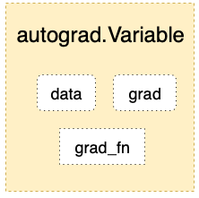
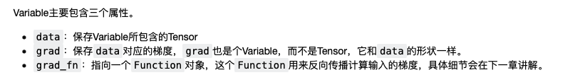
autograd.Variable是Autograd中的核心类，它简单封装了Tensor，并支持几乎所有Tensor有的操作。Tensor在被封装为Variable之后，可以调用它的.backward实现反向传播，自动计算所有梯度。Variable的数据结构如图所示。

from torch.autograd import Variable
# 使用Tensor新建一个Variable
x = Variable(t.ones(2, 2), requires_grad = True)
x
output:
Variable containing:
 1  1
 1  1
[torch.FloatTensor of size 2x2]

y = x.sum()
y
output:
Variable containing:
 4
[torch.FloatTensor of size 1]

y.grad_fn
<SumBackward0 at 0x7fc14824b860>

y.backward() # 反向传播,计算梯度
# y = x.sum() = (x[0][0] + x[0][1] + x[1][0] + x[1][1])
# 每个值的梯度都为1
x.grad 
Variable containing:
 1  1
 1  1
[torch.FloatTensor of size 2x2]

注意：grad在反向传播过程中是累加的(accumulated)，这意味着每一次运行反向传播，梯度都会累加之前的梯度，所以反向传播之前需把梯度清零。

#一次反向传播
y.backward()
x.grad
output：
Variable containing:
 2  2
 2  2
[torch.FloatTensor of size 2x2]
#又一次反向传播
y.backward()
x.grad
output：
Variable containing:
 3  3
 3  3
[torch.FloatTensor of size 2x2]

# 以下划线结束的函数是inplace操作，就像add_
x.grad.data.zero_()
output：
 0  0
 0  0
[torch.FloatTensor of size 2x2]

y.backward()
x.grad
output：
Variable containing:
 1  1
 1  1
[torch.FloatTensor of size 2x2]

Variable和Tensor具有近乎一致的接口，在实际使用中可以无缝切换。

x = Variable(t.ones(4,5))
y = t.cos(x)
x_tensor_cos = t.cos(x.data)
print(y)
x_tensor_cos
output:
Variable containing:
 0.5403  0.5403  0.5403  0.5403  0.5403
 0.5403  0.5403  0.5403  0.5403  0.5403
 0.5403  0.5403  0.5403  0.5403  0.5403
 0.5403  0.5403  0.5403  0.5403  0.5403
[torch.FloatTensor of size 4x5]

Out[25]:

 0.5403  0.5403  0.5403  0.5403  0.5403
 0.5403  0.5403  0.5403  0.5403  0.5403
 0.5403  0.5403  0.5403  0.5403  0.5403
 0.5403  0.5403  0.5403  0.5403  0.5403
[torch.FloatTensor of size 4x5]

神经网络

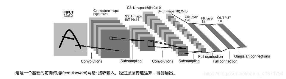
Autograd实现了反向传播功能，但是直接用来写深度学习的代码在很多情况下还是稍显复杂，torch.nn是专门为神经网络设计的模块化接口。nn构建于 Autograd之上，可用来定义和运行神经网络。nn.Module是nn中最重要的类，可把它看成是一个网络的封装，包含网络各层定义以及forward方法，调用forward(input)方法，可返回前向传播的结果。下面就以最早的卷积神经网络：LeNet为例，来看看如何用nn.Module实现。LeNet的网络结构如图所示
在这里插入图片描述

定义网络

定义网络时，需要继承nn.Module，并实现它的forward方法，把网络中具有可学习参数的层放在构造函数__init__中。如果某一层(如ReLU)不具有可学习的参数，则既可以放在构造函数中，也可以不放，但建议不放在其中，而在forward中使用nn.functional代替。

import torch.nn as nn
import torch.nn.functional as F

class Net(nn.Module):
    def __init__(self):
        # nn.Module子类的函数必须在构造函数中执行父类的构造函数
        # 下式等价于nn.Module.__init__(self)
        super(Net, self).__init__()
        
        # 卷积层 '1'表示输入图片为单通道, '6'表示输出通道数，'5'表示卷积核为5*5
        self.conv1 = nn.Conv2d(1, 6, 5) 
        # 卷积层
        self.conv2 = nn.Conv2d(6, 16, 5) 
        # 仿射层/全连接层，y = Wx + b
        self.fc1   = nn.Linear(16*5*5, 120) 
        self.fc2   = nn.Linear(120, 84)
        self.fc3   = nn.Linear(84, 10)

    def forward(self, x): 
        # 卷积 -> 激活 -> 池化 
        x = F.max_pool2d(F.relu(self.conv1(x)), (2, 2))
        x = F.max_pool2d(F.relu(self.conv2(x)), 2) 
        # reshape，‘-1’表示自适应
        x = x.view(x.size()[0], -1) 
        x = F.relu(self.fc1(x))
        x = F.relu(self.fc2(x))
        x = self.fc3(x)        
        return x

net = Net()
print(net)

output：
Net(
  (conv1): Conv2d (1, 6, kernel_size=(5, 5), stride=(1, 1))
  (conv2): Conv2d (6, 16, kernel_size=(5, 5), stride=(1, 1))
  (fc1): Linear(in_features=400, out_features=120)
  (fc2): Linear(in_features=120, out_features=84)
  (fc3): Linear(in_features=84, out_features=10)
)

只要在nn.Module的子类中定义了forward函数，backward函数就会自动被实现(利用Autograd)。在forward 函数中可使用任何Variable支持的函数，还可以使用if、for循环、print、log等Python语法，写法和标准的Python写法一致。
网络的可学习参数通过net.parameters()返回，net.named_parameters可同时返回可学习的参数及名称。

params = list(net.parameters())
print(len(params))
for name,parameters in net.named_parameters():
    print(name,':',parameters.size())

output：
10
conv1.weight : torch.Size([6, 1, 5, 5])
conv1.bias : torch.Size([6])
conv2.weight : torch.Size([16, 6, 5, 5])
conv2.bias : torch.Size([16])
fc1.weight : torch.Size([120, 400])
fc1.bias : torch.Size([120])
fc2.weight : torch.Size([84, 120])
fc2.bias : torch.Size([84])
fc3.weight : torch.Size([10, 84])
fc3.bias : torch.Size([10])

forward函数的输入和输出都是Variable，只有Variable才具有自动求导功能，而Tensor是没有的，所以在输入时，需把Tensor封装成Variable。

input = Variable(t.randn(1, 1, 32, 32).float())
out = net(input)
out.size()

output：
torch.Size([1, 10])

net.zero_grad() # 所有参数的梯度清零
out.backward(Variable(t.ones(1,10))) # 反向传播

在这里插入图片描述

损失函数

nn实现了神经网络中大多数的损失函数，例如nn.MSELoss用来计算均方误差，nn.CrossEntropyLoss用来计算交叉熵损失

output = net(input)
target = Variable(t.arange(0,10).float())  
criterion = nn.MSELoss()
loss = criterion(output, target)
loss

output:
Variable containing:
 28.5536
[torch.FloatTensor of size 1]

在这里插入图片描述

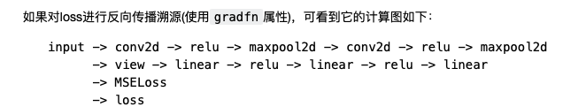
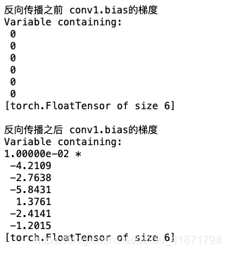
当调用loss.backward()时，该图会动态生成并自动微分，也即会自动计算图中参数(Parameter)的导数。

# 运行.backward，观察调用之前和调用之后的grad
net.zero_grad() # 把net中所有可学习参数的梯度清零
print('反向传播之前 conv1.bias的梯度')
print(net.conv1.bias.grad)
loss.backward()
print('反向传播之后 conv1.bias的梯度')
print(net.conv1.bias.grad)

在这里插入图片描述

优化器

在反向传播计算完所有参数的梯度后，还需要使用优化方法来更新网络的权重和参数，例如随机梯度下降法(SGD)的更新策略如下：

weight = weight - learning_rate * gradient

手动实现如下：

learning_rate = 0.01
for f in net.parameters():
    f.data.sub_(f.grad.data * learning_rate)# inplace 减法

torch.optim中实现了深度学习中绝大多数的优化方法，例如RMSProp、Adam、SGD等，更便于使用，因此大多数时候并不需要手动写上述代码

import torch.optim as optim
#新建一个优化器，指定要调整的参数和学习率
optimizer = optim.SGD(net.parameters(), lr = 0.01)
# 在训练过程中
# 先梯度清零(与net.zero_grad()效果一样)
optimizer.zero_grad() 
# 计算损失
output = net(input)
loss = criterion(output, target)
#反向传播
loss.backward() 
#更新参数
optimizer.step()

数据加载与预处理

在深度学习中数据加载及预处理是非常复杂繁琐的，但PyTorch提供了一些可极大简化和加快数据处理流程的工具。同时，对于常用的数据集，PyTorch也提供了封装好的接口供用户快速调用，这些数据集主要保存在torchvison中。
torchvision实现了常用的图像数据加载功能，例如Imagenet、CIFAR10、MNIST等，以及常用的数据转换操作，这极大地方便了数据加载，并且代码具有可重用性。

CIFAR-10分类

使用torchvision加载并预处理CIFAR-10数据集
定义网络
定义损失函数和优化器
训练网络并更新网络参数
测试网络

CIFAR-10数据加载及预处理

在这里插入图片描述


# 第一次运行程序torchvision会自动下载CIFAR-10数据集，
# 大约100M，需花费一定的时间，
# 如果已经下载有CIFAR-10，可通过root参数指定

# 定义对数据的预处理
transform = transforms.Compose([
        transforms.ToTensor(), # 转为Tensor
        transforms.Normalize((0.5, 0.5, 0.5), (0.5, 0.5, 0.5)), # 归一化
                             ])

# 训练集
trainset = tv.datasets.CIFAR10(
                    root='/Users/lichao/学习资料/研究生阶段/PYTORCH_LEARNING/dataset',
                    train=True, 
                    download=True,
                    transform=transform)

trainloader = t.utils.data.DataLoader(
                    trainset, 
                    batch_size=4,
                    shuffle=True, 
                    num_workers=2)

# 测试集
testset = tv.datasets.CIFAR10(
                    '/Users/lichao/学习资料/研究生阶段/PYTORCH_LEARNING/dataset',
                    train=False, 
                    download=True, 
                    transform=transform)

testloader = t.utils.data.DataLoader(
                    testset,
                    batch_size=4, 
                    shuffle=False,
                    num_workers=2)

classes = ('plane', 'car', 'bird', 'cat',
           'deer', 'dog', 'frog', 'horse', 'ship', 'truck')

Dataset对象是一个数据集，可以按下标访问，返回形如(data, label)的数据。

(data, label) = trainset[500]
print(classes[label])
# (data + 1) / 2是为了还原被归一化的数据
show((data + 1) / 2).resize((100, 100))

Dataloader是一个可迭代的对象，它将dataset返回的每一条数据拼接成一个batch，并提供多线程加速优化和数据打乱等操作。当程序对dataset的所有数据遍历完一遍之后，相应的对Dataloader也完成了一次迭代。

dataiter = iter(trainloader)
images, labels = dataiter.next() # 返回4张图片及标签
print(' '.join('%11s'%classes[labels[j]] for j in range(4)))
show(tv.utils.make_grid((images+1)/2)).resize((400,100))

定义网络


import torch.nn as nn
import torch.nn.functional as F

class Net(nn.Module):
    def __init__(self):
        super(Net, self).__init__()
        self.conv1 = nn.Conv2d(3, 6, 5) 
        self.conv2 = nn.Conv2d(6, 16, 5)  
        self.fc1   = nn.Linear(16*5*5, 120)  
        self.fc2   = nn.Linear(120, 84)
        self.fc3   = nn.Linear(84, 10)

    def forward(self, x): 
        x = F.max_pool2d(F.relu(self.conv1(x)), (2, 2)) 
        x = F.max_pool2d(F.relu(self.conv2(x)), 2) 
        x = x.view(x.size()[0], -1) 
        x = F.relu(self.fc1(x))
        x = F.relu(self.fc2(x))
        x = self.fc3(x)        
        return x
net = Net()
print(net)

定义损失函数和优化器(loss和optimizer)


from torch import optim
criterion = nn.CrossEntropyLoss() # 交叉熵损失函数
optimizer = optim.SGD(net.parameters(), lr=0.001, momentum=0.9)

训练网络

输入数据
前向传播+反向传播
更新参数

t.set_num_threads(8)
for epoch in range(2):  
    running_loss = 0.0
    for i, data in enumerate(trainloader, 0):
        
        # 输入数据
        inputs, labels = data
        inputs, labels = Variable(inputs), Variable(labels)
        
        # 梯度清零
        optimizer.zero_grad()
        
        # forward + backward 
        outputs = net(inputs)
        loss = criterion(outputs, labels)
        loss.backward()   
        
        # 更新参数 
        optimizer.step()
        
        # 打印log信息
        running_loss += loss.item()
        if i % 2000 == 1999: # 每2000个batch打印一下训练状态
            print('[%d, %5d] loss: %.3f' \
                  % (epoch+1, i+1, running_loss / 2000))
            running_loss = 0.0
print('Finished Training')

此处仅训练了2个epoch（遍历完一遍数据集称为一个epoch），来看看网络有没有效果。将测试图片输入到网络中，计算它的label，然后与实际的label进行比较。

dataiter = iter(testloader)
images, labels = dataiter.next() # 一个batch返回4张图片
print('实际的label: ', ' '.join(\
            '%08s'%classes[labels[j]] for j in range(4)))
show(tv.utils.make_grid(images / 2 - 0.5)).resize((400,100))

接着计算网络预测的label：

# 计算图片在每个类别上的分数
outputs = net(Variable(images))
# 得分最高的那个类
_, predicted = t.max(outputs.data, 1)

print('预测结果: ', ' '.join('%5s'\
            % classes[predicted[j]] for j in range(4)))

看看在整个测试集上的效果

correct = 0 # 预测正确的图片数
total = 0 # 总共的图片数
for data in testloader:
    images, labels = data
    outputs = net(Variable(images))
    _, predicted = t.max(outputs.data, 1)
    total += labels.size(0)
    correct += (predicted == labels).sum()
print('10000张测试集中的准确率为: %d %%' % (100 * correct / total))

在GPU训练

就像之前把Tensor从CPU转到GPU一样，模型也可以类似地从CPU转到GPU。

#%%
if t.cuda.is_available():
    net.cuda()
    images = images.cuda()
    labels = labels.cuda()
    output = net(Variable(images))
    loss= criterion(output,Variable(labels))

如果发现在GPU上并没有比CPU提速很多，实际上是因为网络比较小，GPU没有完全发挥自己的真正实力。